Finding the MSD uncertainties from a VASP file

Using kinisi to obtain the mean-squared displacement and uncertainty in a VASP Xdatcar type file is straightforward and involves using the DiffusionAnalyzer class.

import numpy as np
from kinisi.analyze import DiffusionAnalyzer
np.random.seed(1)

There the params dictionary describes details about the simulation, and are fully documented in the parser module. The 'specie' is the atomic/ionic species that you want to calculate the MSD for, the 'time_step' is the simulation timestep in your molecular dynamics, and the 'step_skip' is the frequency which with the data was written in your simulation trajectory.

params = {'specie': 'Li',
          'time_step': 2.0,
          'step_skip': 50}

Therefore, for this example, we have a simulation that had a timestep of 2 femtoseconds (note the FAQs about units) but we only stored the trajectory information every 50 steps and we want to investigate only the lithium motion.

msd = DiffusionAnalyzer.from_file('example_XDATCAR.gz', parser_params=params)

Reading Trajectory: 0%| | 0/140 [00:00<?, ?it/s]

</pre>

Reading Trajectory: 0%| | 0/140 [00:00<?, ?it/s]

end{sphinxVerbatim}

Reading Trajectory: 0%| | 0/140 [00:00<?, ?it/s]

Reading Trajectory: 100%|██████████| 140/140 [00:00&lt;00:00, 4277.59it/s]

</pre>

Reading Trajectory: 100%|██████████| 140/140 [00:00<00:00, 4277.59it/s]

end{sphinxVerbatim}

Reading Trajectory: 100%|██████████| 140/140 [00:00<00:00, 4277.59it/s]

Getting Displacements: 0%| | 0/100 [00:00&lt;?, ?it/s]

</pre>

Getting Displacements: 0%| | 0/100 [00:00<?, ?it/s]

end{sphinxVerbatim}

Getting Displacements: 0%| | 0/100 [00:00<?, ?it/s]

Getting Displacements: 100%|██████████| 100/100 [00:00&lt;00:00, 16198.60it/s]

</pre>

Getting Displacements: 100%|██████████| 100/100 [00:00<00:00, 16198.60it/s]

end{sphinxVerbatim}

Getting Displacements: 100%|██████████| 100/100 [00:00<00:00, 16198.60it/s]

Finding Means and Variances: 0%| | 0/100 [00:00&lt;?, ?it/s]

</pre>

Finding Means and Variances: 0%| | 0/100 [00:00<?, ?it/s]

end{sphinxVerbatim}

Finding Means and Variances: 0%| | 0/100 [00:00<?, ?it/s]

Finding Means and Variances: 14%|█▍ | 14/100 [00:00&lt;00:00, 132.41it/s]

</pre>

Finding Means and Variances: 14%|█▍ | 14/100 [00:00<00:00, 132.41it/s]

end{sphinxVerbatim}

Finding Means and Variances: 14%|█▍ | 14/100 [00:00<00:00, 132.41it/s]

Finding Means and Variances: 28%|██▊ | 28/100 [00:00&lt;00:00, 132.26it/s]

</pre>

Finding Means and Variances: 28%|██▊ | 28/100 [00:00<00:00, 132.26it/s]

end{sphinxVerbatim}

Finding Means and Variances: 28%|██▊ | 28/100 [00:00<00:00, 132.26it/s]

Finding Means and Variances: 42%|████▏ | 42/100 [00:00&lt;00:00, 132.55it/s]

</pre>

Finding Means and Variances: 42%|████▏ | 42/100 [00:00<00:00, 132.55it/s]

end{sphinxVerbatim}

Finding Means and Variances: 42%|████▏ | 42/100 [00:00<00:00, 132.55it/s]

Finding Means and Variances: 56%|█████▌ | 56/100 [00:00&lt;00:00, 134.53it/s]

</pre>

Finding Means and Variances: 56%|█████▌ | 56/100 [00:00<00:00, 134.53it/s]

end{sphinxVerbatim}

Finding Means and Variances: 56%|█████▌ | 56/100 [00:00<00:00, 134.53it/s]

Finding Means and Variances: 71%|███████ | 71/100 [00:00&lt;00:00, 138.92it/s]

</pre>

Finding Means and Variances: 71%|███████ | 71/100 [00:00<00:00, 138.92it/s]

end{sphinxVerbatim}

Finding Means and Variances: 71%|███████ | 71/100 [00:00<00:00, 138.92it/s]

Finding Means and Variances: 93%|█████████▎| 93/100 [00:00&lt;00:00, 165.19it/s]

</pre>

Finding Means and Variances: 93%|█████████▎| 93/100 [00:00<00:00, 165.19it/s]

end{sphinxVerbatim}

Finding Means and Variances: 93%|█████████▎| 93/100 [00:00<00:00, 165.19it/s]

Finding Means and Variances: 100%|██████████| 100/100 [00:00&lt;00:00, 154.41it/s]

</pre>

Finding Means and Variances: 100%|██████████| 100/100 [00:00<00:00, 154.41it/s]

end{sphinxVerbatim}

Finding Means and Variances: 100%|██████████| 100/100 [00:00<00:00, 154.41it/s]

The DiffusionAnalyzer will perform the bootstrapping process to obtain the displacements and uncertainties (this is detailed in the methodology. To find out how to determine the diffusion coefficient with DiffusionAnalyzer continue here.

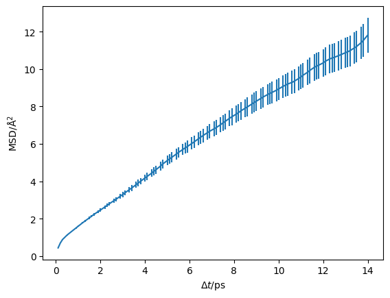
Then the MSD (msd) as a function of timestep (dt) can be plotted.

import matplotlib.pyplot as plt

plt.errorbar(msd.dt, msd.msd, msd.msd_std)
plt.ylabel('MSD/Å$^2$')
plt.xlabel('$\Delta t$/ps')
plt.show()