Diffusion coefficient from a VASP file#
Previously, we looked at obtaining accurate estimates for the mean-squared displacement with kinisi. Here, we show using the same class to evaluate the diffusion coefficient, using the kinisi methodology.
[1]:
import numpy as np
from kinisi.analyze import DiffusionAnalyzer
from pymatgen.io.vasp import Xdatcar
np.random.seed(42)
rng = np.random.RandomState(42)
There the p_params dictionary describes details about the simulation, and are documented in the parser module (also see the MSD Notebook).
[2]:
p_params = {'specie': 'Li',
            'time_step': 2.0,
            'step_skip': 50}
While the b_params dictionary describes the details of the bootstrapping process, these are documented in the diffusion module. Here, we indicate that we only want to investigate diffusion in the xy-plane of the system.
[3]:
u_params = {'dimension': 'xy'}
[4]:
xd = Xdatcar('./example_XDATCAR.gz')
diff = DiffusionAnalyzer.from_Xdatcar(xd, parser_params=p_params, uncertainty_params=u_params)
- Reading Trajectory: 0%| | 0/140 [00:00<?, ?it/s]
</pre>
- Reading Trajectory: 0%| | 0/140 [00:00<?, ?it/s]
end{sphinxVerbatim}
Reading Trajectory: 0%| | 0/140 [00:00<?, ?it/s]
- Reading Trajectory: 100%|██████████| 140/140 [00:00<00:00, 4387.25it/s]
</pre>
- Reading Trajectory: 100%|██████████| 140/140 [00:00<00:00, 4387.25it/s]
end{sphinxVerbatim}
Reading Trajectory: 100%|██████████| 140/140 [00:00<00:00, 4387.25it/s]
- Getting Displacements: 0%| | 0/100 [00:00<?, ?it/s]
</pre>
- Getting Displacements: 0%| | 0/100 [00:00<?, ?it/s]
end{sphinxVerbatim}
Getting Displacements: 0%| | 0/100 [00:00<?, ?it/s]
- Getting Displacements: 100%|██████████| 100/100 [00:00<00:00, 16174.86it/s]
</pre>
- Getting Displacements: 100%|██████████| 100/100 [00:00<00:00, 16174.86it/s]
end{sphinxVerbatim}
Getting Displacements: 100%|██████████| 100/100 [00:00<00:00, 16174.86it/s]
- Finding Means and Variances: 0%| | 0/100 [00:00<?, ?it/s]
</pre>
- Finding Means and Variances: 0%| | 0/100 [00:00<?, ?it/s]
end{sphinxVerbatim}
Finding Means and Variances: 0%| | 0/100 [00:00<?, ?it/s]
- Finding Means and Variances: 12%|█▏ | 12/100 [00:00<00:00, 112.27it/s]
</pre>
- Finding Means and Variances: 12%|█▏ | 12/100 [00:00<00:00, 112.27it/s]
end{sphinxVerbatim}
Finding Means and Variances: 12%|█▏ | 12/100 [00:00<00:00, 112.27it/s]
- Finding Means and Variances: 24%|██▍ | 24/100 [00:00<00:00, 107.80it/s]
</pre>
- Finding Means and Variances: 24%|██▍ | 24/100 [00:00<00:00, 107.80it/s]
end{sphinxVerbatim}
Finding Means and Variances: 24%|██▍ | 24/100 [00:00<00:00, 107.80it/s]
- Finding Means and Variances: 36%|███▌ | 36/100 [00:00<00:00, 109.11it/s]
</pre>
- Finding Means and Variances: 36%|███▌ | 36/100 [00:00<00:00, 109.11it/s]
end{sphinxVerbatim}
Finding Means and Variances: 36%|███▌ | 36/100 [00:00<00:00, 109.11it/s]
- Finding Means and Variances: 49%|████▉ | 49/100 [00:00<00:00, 113.69it/s]
</pre>
- Finding Means and Variances: 49%|████▉ | 49/100 [00:00<00:00, 113.69it/s]
end{sphinxVerbatim}
Finding Means and Variances: 49%|████▉ | 49/100 [00:00<00:00, 113.69it/s]
- Finding Means and Variances: 61%|██████ | 61/100 [00:00<00:00, 115.71it/s]
</pre>
- Finding Means and Variances: 61%|██████ | 61/100 [00:00<00:00, 115.71it/s]
end{sphinxVerbatim}
Finding Means and Variances: 61%|██████ | 61/100 [00:00<00:00, 115.71it/s]
- Finding Means and Variances: 74%|███████▍ | 74/100 [00:00<00:00, 119.42it/s]
</pre>
- Finding Means and Variances: 74%|███████▍ | 74/100 [00:00<00:00, 119.42it/s]
end{sphinxVerbatim}
Finding Means and Variances: 74%|███████▍ | 74/100 [00:00<00:00, 119.42it/s]
- Finding Means and Variances: 99%|█████████▉| 99/100 [00:00<00:00, 159.39it/s]
</pre>
- Finding Means and Variances: 99%|█████████▉| 99/100 [00:00<00:00, 159.39it/s]
end{sphinxVerbatim}
Finding Means and Variances: 99%|█████████▉| 99/100 [00:00<00:00, 159.39it/s]
- Finding Means and Variances: 100%|██████████| 100/100 [00:00<00:00, 133.50it/s]
</pre>
- Finding Means and Variances: 100%|██████████| 100/100 [00:00<00:00, 133.50it/s]
end{sphinxVerbatim}
Finding Means and Variances: 100%|██████████| 100/100 [00:00<00:00, 133.50it/s]
In the above cells, we parse and determine the uncertainty on the mean-squared displacement as a function of the timestep. We should visualise this, to check that we are observing diffusion in our material and to determine the timescale at which this diffusion begins.
[5]:
import matplotlib.pyplot as plt
[6]:
plt.errorbar(diff.dt, diff.msd, diff.msd_std)
plt.ylabel('MSD/Å$^2$')
plt.xlabel('$\Delta t$/ps')
plt.show()
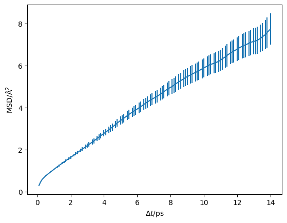
We can visualise this on a log-log scale, which helps to reveal the diffusive regime (the region where the gradient stops changing).
[7]:
plt.errorbar(diff.dt, diff.msd, diff.msd_std)
plt.axvline(2, color='g')
plt.ylabel('MSD/Å$^2$')
plt.xlabel('$\Delta t$/ps')
plt.yscale('log')
plt.xscale('log')
plt.show()
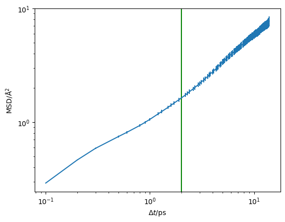
The green line at 2 ps appears to be a reasonable estimate of the start of the diffusive regime. Therefore, we want to pass 2 as the argument to the diffusion analysis below.
[8]:
diff.diffusion(2, diffusion_params={'random_state': rng})
/home/docs/checkouts/readthedocs.org/user_builds/kinisi/envs/latest/lib/python3.9/site-packages/scipy/optimize/_numdiff.py:590: RuntimeWarning: invalid value encountered in subtract
  df = fun(x) - f0
- Likelihood Sampling: 0%| | 0/1500 [00:00<?, ?it/s]
</pre>
- Likelihood Sampling: 0%| | 0/1500 [00:00<?, ?it/s]
end{sphinxVerbatim}
Likelihood Sampling: 0%| | 0/1500 [00:00<?, ?it/s]
- Likelihood Sampling: 2%|▏ | 34/1500 [00:00<00:04, 335.83it/s]
</pre>
- Likelihood Sampling: 2%|▏ | 34/1500 [00:00<00:04, 335.83it/s]
end{sphinxVerbatim}
Likelihood Sampling: 2%|▏ | 34/1500 [00:00<00:04, 335.83it/s]
- Likelihood Sampling: 8%|▊ | 121/1500 [00:00<00:02, 646.19it/s]
</pre>
- Likelihood Sampling: 8%|▊ | 121/1500 [00:00<00:02, 646.19it/s]
end{sphinxVerbatim}
Likelihood Sampling: 8%|▊ | 121/1500 [00:00<00:02, 646.19it/s]
- Likelihood Sampling: 14%|█▍ | 210/1500 [00:00<00:01, 756.09it/s]
</pre>
- Likelihood Sampling: 14%|█▍ | 210/1500 [00:00<00:01, 756.09it/s]
end{sphinxVerbatim}
Likelihood Sampling: 14%|█▍ | 210/1500 [00:00<00:01, 756.09it/s]
- Likelihood Sampling: 20%|█▉ | 298/1500 [00:00<00:01, 804.06it/s]
</pre>
- Likelihood Sampling: 20%|█▉ | 298/1500 [00:00<00:01, 804.06it/s]
end{sphinxVerbatim}
Likelihood Sampling: 20%|█▉ | 298/1500 [00:00<00:01, 804.06it/s]
- Likelihood Sampling: 26%|██▌ | 387/1500 [00:00<00:01, 834.16it/s]
</pre>
- Likelihood Sampling: 26%|██▌ | 387/1500 [00:00<00:01, 834.16it/s]
end{sphinxVerbatim}
Likelihood Sampling: 26%|██▌ | 387/1500 [00:00<00:01, 834.16it/s]
- Likelihood Sampling: 31%|███▏ | 472/1500 [00:00<00:01, 836.95it/s]
</pre>
- Likelihood Sampling: 31%|███▏ | 472/1500 [00:00<00:01, 836.95it/s]
end{sphinxVerbatim}
Likelihood Sampling: 31%|███▏ | 472/1500 [00:00<00:01, 836.95it/s]
- Likelihood Sampling: 37%|███▋ | 562/1500 [00:00<00:01, 855.59it/s]
</pre>
- Likelihood Sampling: 37%|███▋ | 562/1500 [00:00<00:01, 855.59it/s]
end{sphinxVerbatim}
Likelihood Sampling: 37%|███▋ | 562/1500 [00:00<00:01, 855.59it/s]
- Likelihood Sampling: 43%|████▎ | 650/1500 [00:00<00:00, 863.09it/s]
</pre>
- Likelihood Sampling: 43%|████▎ | 650/1500 [00:00<00:00, 863.09it/s]
end{sphinxVerbatim}
Likelihood Sampling: 43%|████▎ | 650/1500 [00:00<00:00, 863.09it/s]
- Likelihood Sampling: 49%|████▉ | 739/1500 [00:00<00:00, 871.27it/s]
</pre>
- Likelihood Sampling: 49%|████▉ | 739/1500 [00:00<00:00, 871.27it/s]
end{sphinxVerbatim}
Likelihood Sampling: 49%|████▉ | 739/1500 [00:00<00:00, 871.27it/s]
- Likelihood Sampling: 55%|█████▌ | 829/1500 [00:01<00:00, 877.34it/s]
</pre>
- Likelihood Sampling: 55%|█████▌ | 829/1500 [00:01<00:00, 877.34it/s]
end{sphinxVerbatim}
Likelihood Sampling: 55%|█████▌ | 829/1500 [00:01<00:00, 877.34it/s]
- Likelihood Sampling: 61%|██████▏ | 919/1500 [00:01<00:00, 882.97it/s]
</pre>
- Likelihood Sampling: 61%|██████▏ | 919/1500 [00:01<00:00, 882.97it/s]
end{sphinxVerbatim}
Likelihood Sampling: 61%|██████▏ | 919/1500 [00:01<00:00, 882.97it/s]
- Likelihood Sampling: 67%|██████▋ | 1008/1500 [00:01<00:00, 880.93it/s]
</pre>
- Likelihood Sampling: 67%|██████▋ | 1008/1500 [00:01<00:00, 880.93it/s]
end{sphinxVerbatim}
Likelihood Sampling: 67%|██████▋ | 1008/1500 [00:01<00:00, 880.93it/s]
- Likelihood Sampling: 73%|███████▎ | 1098/1500 [00:01<00:00, 884.86it/s]
</pre>
- Likelihood Sampling: 73%|███████▎ | 1098/1500 [00:01<00:00, 884.86it/s]
end{sphinxVerbatim}
Likelihood Sampling: 73%|███████▎ | 1098/1500 [00:01<00:00, 884.86it/s]
- Likelihood Sampling: 79%|███████▉ | 1187/1500 [00:01<00:00, 884.96it/s]
</pre>
- Likelihood Sampling: 79%|███████▉ | 1187/1500 [00:01<00:00, 884.96it/s]
end{sphinxVerbatim}
Likelihood Sampling: 79%|███████▉ | 1187/1500 [00:01<00:00, 884.96it/s]
- Likelihood Sampling: 85%|████████▌ | 1277/1500 [00:01<00:00, 888.53it/s]
</pre>
- Likelihood Sampling: 85%|████████▌ | 1277/1500 [00:01<00:00, 888.53it/s]
end{sphinxVerbatim}
Likelihood Sampling: 85%|████████▌ | 1277/1500 [00:01<00:00, 888.53it/s]
- Likelihood Sampling: 91%|█████████ | 1367/1500 [00:01<00:00, 890.92it/s]
</pre>
- Likelihood Sampling: 91%|█████████ | 1367/1500 [00:01<00:00, 890.92it/s]
end{sphinxVerbatim}
Likelihood Sampling: 91%|█████████ | 1367/1500 [00:01<00:00, 890.92it/s]
- Likelihood Sampling: 97%|█████████▋| 1457/1500 [00:01<00:00, 888.20it/s]
</pre>
- Likelihood Sampling: 97%|█████████▋| 1457/1500 [00:01<00:00, 888.20it/s]
end{sphinxVerbatim}
Likelihood Sampling: 97%|█████████▋| 1457/1500 [00:01<00:00, 888.20it/s]
- Likelihood Sampling: 100%|██████████| 1500/1500 [00:01<00:00, 851.15it/s]
</pre>
- Likelihood Sampling: 100%|██████████| 1500/1500 [00:01<00:00, 851.15it/s]
end{sphinxVerbatim}
Likelihood Sampling: 100%|██████████| 1500/1500 [00:01<00:00, 851.15it/s]
This method estimates the correlation matrix between the timesteps and uses likelihood sampling to find the diffusion coefficient, \(D\) and intercept (the units are cm :sup:2 /s and Å :sup:2 respectively). Now we can probe these objects.
We can get the median and 95 % confidence interval using,
[9]:
diff.D.n, diff.D.ci()
[9]:
(1.398949947861664e-05, array([1.21269232e-05, 1.59063930e-05]))
[10]:
diff.intercept.n, diff.intercept.ci()
[10]:
(0.5108225828314326, array([0.37880864, 0.64024882]))
Or we can get all of the sampled values from one of these objects.
[11]:
diff.D.samples
[11]:
array([1.43149306e-05, 1.41068282e-05, 1.35887732e-05, ...,
       1.43490124e-05, 1.54446286e-05, 1.39840873e-05])
Having completed the analysis, we can save the object for use later (such as downstream by a plotting script).
[13]:
diff.save('example.hdf')
The data is saved in a HDF5 file format which helps us efficiently store our data. We can then load the data with the following class method.
[14]:
loaded_diff = DiffusionAnalyzer.load('example.hdf')
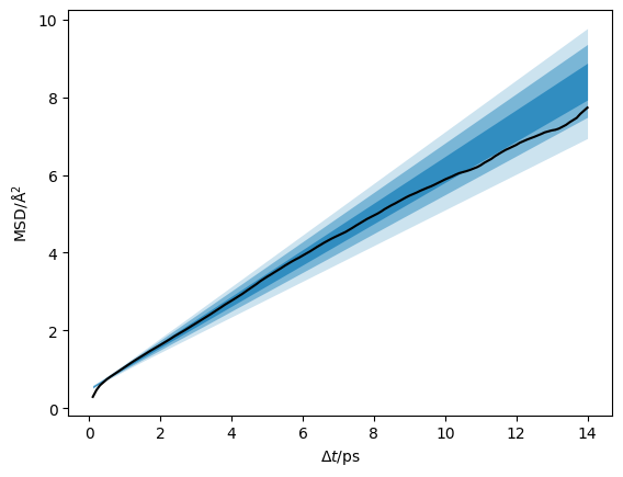
We can plot the data with the credible intervals from the \(D\) and \(D_{\text{offset}}\) distribution.
[15]:
credible_intervals = [[16, 84], [2.5, 97.5], [0.15, 99.85]]
alpha = [0.6, 0.4, 0.2]

plt.plot(loaded_diff.dt, loaded_diff.msd, 'k-')
for i, ci in enumerate(credible_intervals):
    plt.fill_between(loaded_diff.dt,
                     *np.percentile(loaded_diff.distribution, ci, axis=1),
                     alpha=alpha[i],
                     color='#0173B2',
                     lw=0)
plt.ylabel('MSD/Å$^2$')
plt.xlabel('$\Delta t$/ps')
plt.show()
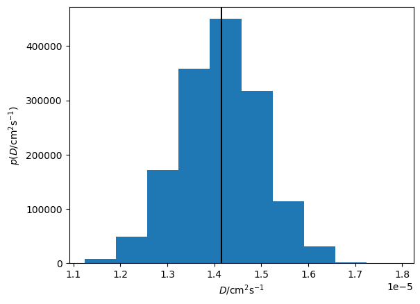
Additionally, we can visualise the distribution of the diffusion coefficient that has been determined.
[16]:
plt.hist(loaded_diff.D.samples, density=True)
plt.axvline(loaded_diff.D.n, c='k')
plt.xlabel('$D$/cm$^2$s$^{-1}$')
plt.ylabel('$p(D$/cm$^2$s$^{-1})$')
plt.show()
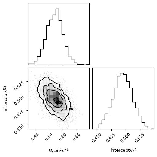
Or the joint probability distribution for the diffusion coefficient and intercept.
[17]:
from corner import corner
[18]:
corner(loaded_diff.flatchain, labels=['$D$/cm$^2$s$^{-1}$', 'intercept/Å$^2$'])
plt.show()
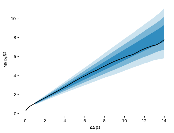
Above, the posterior distribution is plotted as a function of \(\Delta t\). kinisi can also compute the posterior predictive distribution of mean-squared displacement data that would be expected from simulations, given the set of linear models for the ensemble MSD described by the posterior distribution, above. Calculating this posterior predictive distribution involves an additional sampling procedure that samples
probable simulated MSDs for each of the probable linear models in the (previously sampled) posterior distribution. The posterior predictive distribution captures uncertainty in the true ensemble MSD and uncertainty in the simulated MSD data expected for each ensemble MSD model, and so has a larger variance than the ensemble MSD posterior distribution.
[19]:
ppd = loaded_diff.posterior_predictive({'n_posterior_samples': 128,
                                        'progress': False})
[20]:
plt.plot(loaded_diff.dt, loaded_diff.msd, 'k-')
for i, ci in enumerate(credible_intervals):
    plt.fill_between(loaded_diff.dt[14:],
                     *np.percentile(ppd.T, ci, axis=1),
                     alpha=alpha[i],
                     color='#0173B2',
                     lw=0)
plt.ylabel('MSD/Å$^2$')
plt.xlabel('$\Delta t$/ps')
plt.show()
