Jump diffusion coefficient from a VASP file#
Previously, we looked at obtaining accurate estimates for the mean-squared displacement with kinisi. Here, we show using the same class to evaluate the diffusion coefficient, using the kinisi methodology.
[1]:
import numpy as np
from kinisi.analyze import JumpDiffusionAnalyzer
from pymatgen.io.vasp import Xdatcar
np.random.seed(42)
rng = np.random.RandomState(42)
There the p_params dictionary describes details about the simulation, and are documented in the parser module (also see the MSD Notebook).
[2]:
p_params = {'specie': 'Li',
            'time_step': 2.0,
            'step_skip': 50}
While the u_params dictionary describes the details of the uncertainty calculation process, these are documented in the diffusion module. Here, we indicate that we only want to investigate diffusion in the xy-plane of the system.
[3]:
u_params = {'dimension': 'xy'}
[4]:
xd = Xdatcar('./example_XDATCAR.gz')
diff = JumpDiffusionAnalyzer.from_Xdatcar(xd, parser_params=p_params, uncertainty_params=u_params)
- Reading Trajectory: 0%| | 0/140 [00:00<?, ?it/s]
</pre>
- Reading Trajectory: 0%| | 0/140 [00:00<?, ?it/s]
end{sphinxVerbatim}
Reading Trajectory: 0%| | 0/140 [00:00<?, ?it/s]
- Reading Trajectory: 100%|██████████| 140/140 [00:00<00:00, 4546.04it/s]
</pre>
- Reading Trajectory: 100%|██████████| 140/140 [00:00<00:00, 4546.04it/s]
end{sphinxVerbatim}
Reading Trajectory: 100%|██████████| 140/140 [00:00<00:00, 4546.04it/s]
- Getting Displacements: 0%| | 0/100 [00:00<?, ?it/s]
</pre>
- Getting Displacements: 0%| | 0/100 [00:00<?, ?it/s]
end{sphinxVerbatim}
Getting Displacements: 0%| | 0/100 [00:00<?, ?it/s]
- Getting Displacements: 100%|██████████| 100/100 [00:00<00:00, 17961.22it/s]
</pre>
- Getting Displacements: 100%|██████████| 100/100 [00:00<00:00, 17961.22it/s]
end{sphinxVerbatim}
Getting Displacements: 100%|██████████| 100/100 [00:00<00:00, 17961.22it/s]
- Finding Means and Variances: 0%| | 0/50 [00:00<?, ?it/s]
</pre>
- Finding Means and Variances: 0%| | 0/50 [00:00<?, ?it/s]
end{sphinxVerbatim}
Finding Means and Variances: 0%| | 0/50 [00:00<?, ?it/s]
- Finding Means and Variances: 30%|███ | 15/50 [00:00<00:00, 141.44it/s]
</pre>
- Finding Means and Variances: 30%|███ | 15/50 [00:00<00:00, 141.44it/s]
end{sphinxVerbatim}
Finding Means and Variances: 30%|███ | 15/50 [00:00<00:00, 141.44it/s]
- Finding Means and Variances: 60%|██████ | 30/50 [00:00<00:00, 141.70it/s]
</pre>
- Finding Means and Variances: 60%|██████ | 30/50 [00:00<00:00, 141.70it/s]
end{sphinxVerbatim}
Finding Means and Variances: 60%|██████ | 30/50 [00:00<00:00, 141.70it/s]
- Finding Means and Variances: 90%|█████████ | 45/50 [00:00<00:00, 144.87it/s]
</pre>
- Finding Means and Variances: 90%|█████████ | 45/50 [00:00<00:00, 144.87it/s]
end{sphinxVerbatim}
Finding Means and Variances: 90%|█████████ | 45/50 [00:00<00:00, 144.87it/s]
- Finding Means and Variances: 100%|██████████| 50/50 [00:00<00:00, 144.74it/s]
</pre>
- Finding Means and Variances: 100%|██████████| 50/50 [00:00<00:00, 144.74it/s]
end{sphinxVerbatim}
Finding Means and Variances: 100%|██████████| 50/50 [00:00<00:00, 144.74it/s]
In the above cells, we parse and determine the uncertainty on the mean-squared displacement as a function of the timestep. We should visualise this, to check that we are observing diffusion in our material and to determine the timescale at which this diffusion begins.
[5]:
import matplotlib.pyplot as plt
[6]:
plt.errorbar(diff.dt, diff.mstd, diff.mstd_std)
plt.ylabel('MSD/Å$^2$')
plt.xlabel('$\Delta t$/ps')
plt.show()
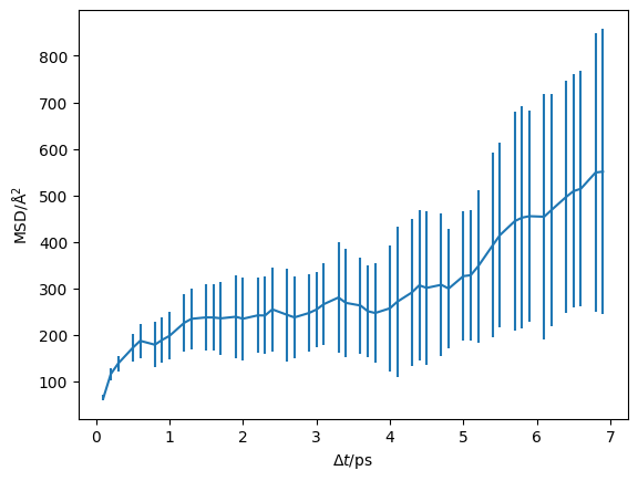
The vertical green line indicates the start of the diffusive regime, based on the maximum of the non-Gaussian parameter. We can also visualise this on a log-log scale, which helps to reveal the diffusive regime.
[7]:
plt.errorbar(diff.dt, diff.mstd, diff.mstd_std)
plt.axvline(4, color='g')
plt.ylabel('MSD/Å$^2$')
plt.xlabel('$\Delta t$/ps')
plt.yscale('log')
plt.xscale('log')
plt.show()
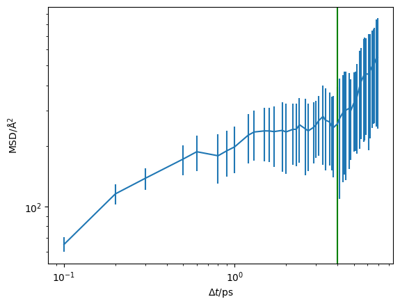
We will set the start of the diffusive regime to be 4 ps using the argument of 4.
[8]:
diff.jump_diffusion(4, jump_diffusion_params={'random_state': rng})
/home/docs/checkouts/readthedocs.org/user_builds/kinisi/envs/latest/lib/python3.9/site-packages/scipy/optimize/_numdiff.py:590: RuntimeWarning: invalid value encountered in subtract
  df = fun(x) - f0
- Likelihood Sampling: 0%| | 0/1500 [00:00<?, ?it/s]
</pre>
- Likelihood Sampling: 0%| | 0/1500 [00:00<?, ?it/s]
end{sphinxVerbatim}
Likelihood Sampling: 0%| | 0/1500 [00:00<?, ?it/s]
- Likelihood Sampling: 9%|▉ | 135/1500 [00:00<00:01, 1344.79it/s]
</pre>
- Likelihood Sampling: 9%|▉ | 135/1500 [00:00<00:01, 1344.79it/s]
end{sphinxVerbatim}
Likelihood Sampling: 9%|▉ | 135/1500 [00:00<00:01, 1344.79it/s]
- Likelihood Sampling: 18%|█▊ | 270/1500 [00:00<00:00, 1346.54it/s]
</pre>
- Likelihood Sampling: 18%|█▊ | 270/1500 [00:00<00:00, 1346.54it/s]
end{sphinxVerbatim}
Likelihood Sampling: 18%|█▊ | 270/1500 [00:00<00:00, 1346.54it/s]
- Likelihood Sampling: 27%|██▋ | 406/1500 [00:00<00:00, 1350.62it/s]
</pre>
- Likelihood Sampling: 27%|██▋ | 406/1500 [00:00<00:00, 1350.62it/s]
end{sphinxVerbatim}
Likelihood Sampling: 27%|██▋ | 406/1500 [00:00<00:00, 1350.62it/s]
- Likelihood Sampling: 36%|███▌ | 543/1500 [00:00<00:00, 1354.84it/s]
</pre>
- Likelihood Sampling: 36%|███▌ | 543/1500 [00:00<00:00, 1354.84it/s]
end{sphinxVerbatim}
Likelihood Sampling: 36%|███▌ | 543/1500 [00:00<00:00, 1354.84it/s]
- Likelihood Sampling: 45%|████▌ | 680/1500 [00:00<00:00, 1359.23it/s]
</pre>
- Likelihood Sampling: 45%|████▌ | 680/1500 [00:00<00:00, 1359.23it/s]
end{sphinxVerbatim}
Likelihood Sampling: 45%|████▌ | 680/1500 [00:00<00:00, 1359.23it/s]
- Likelihood Sampling: 54%|█████▍ | 817/1500 [00:00<00:00, 1362.21it/s]
</pre>
- Likelihood Sampling: 54%|█████▍ | 817/1500 [00:00<00:00, 1362.21it/s]
end{sphinxVerbatim}
Likelihood Sampling: 54%|█████▍ | 817/1500 [00:00<00:00, 1362.21it/s]
- Likelihood Sampling: 64%|██████▎ | 954/1500 [00:00<00:00, 1362.53it/s]
</pre>
- Likelihood Sampling: 64%|██████▎ | 954/1500 [00:00<00:00, 1362.53it/s]
end{sphinxVerbatim}
Likelihood Sampling: 64%|██████▎ | 954/1500 [00:00<00:00, 1362.53it/s]
- Likelihood Sampling: 73%|███████▎ | 1091/1500 [00:00<00:00, 1361.22it/s]
</pre>
- Likelihood Sampling: 73%|███████▎ | 1091/1500 [00:00<00:00, 1361.22it/s]
end{sphinxVerbatim}
Likelihood Sampling: 73%|███████▎ | 1091/1500 [00:00<00:00, 1361.22it/s]
- Likelihood Sampling: 82%|████████▏ | 1228/1500 [00:00<00:00, 1363.61it/s]
</pre>
- Likelihood Sampling: 82%|████████▏ | 1228/1500 [00:00<00:00, 1363.61it/s]
end{sphinxVerbatim}
Likelihood Sampling: 82%|████████▏ | 1228/1500 [00:00<00:00, 1363.61it/s]
- Likelihood Sampling: 91%|█████████ | 1365/1500 [00:01<00:00, 1360.03it/s]
</pre>
- Likelihood Sampling: 91%|█████████ | 1365/1500 [00:01<00:00, 1360.03it/s]
end{sphinxVerbatim}
Likelihood Sampling: 91%|█████████ | 1365/1500 [00:01<00:00, 1360.03it/s]
- Likelihood Sampling: 100%|██████████| 1500/1500 [00:01<00:00, 1358.44it/s]
</pre>
- Likelihood Sampling: 100%|██████████| 1500/1500 [00:01<00:00, 1358.44it/s]
end{sphinxVerbatim}
Likelihood Sampling: 100%|██████████| 1500/1500 [00:01<00:00, 1358.44it/s]
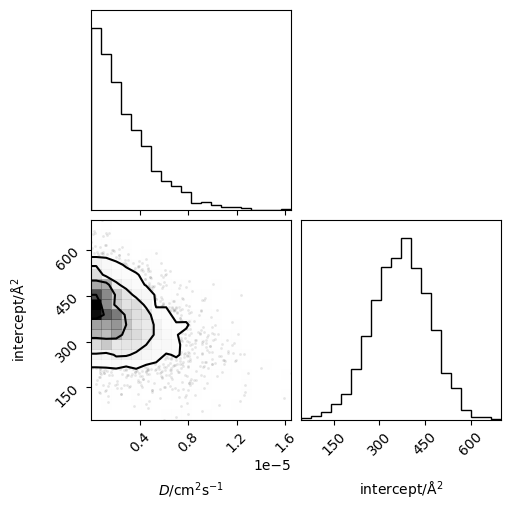
This method estimates the correlation matrix between the timesteps and uses likelihood sampling to find the diffusion coefficient, \(D\) and intercept (the units are cm :sup:2 /s and Å :sup:2 respectively). Now we can probe these objects.
We can get the median and 95 % confidence interval using,
[9]:
diff.D_J.n, diff.D_J.con_int()
[9]:
(2.1766286388198055e-06, array([7.90598621e-08, 8.99636135e-06]))
[10]:
diff.intercept.n, diff.intercept.con_int()
[10]:
(374.7679204791584, array([182.61242932, 548.81354053]))
Or we can get all of the sampled values from one of these objects.
[11]:
diff.D_J.samples
[11]:
array([1.93618828e-06, 4.28496919e-06, 5.02390673e-06, ...,
       2.90798171e-06, 1.90111467e-06, 6.10068311e-06])
Having completed the analysis, we can save the object for use later (such as downstream by a plotting script).
[13]:
diff.save('example.hdf')
The data is saved in a HDF5 file format which helps us efficiently store our data. We can then load the data with the following class method.
[14]:
loaded_diff = JumpDiffusionAnalyzer.load('example.hdf')
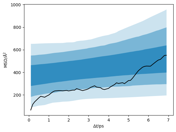
We can plot the data with the credible intervals from the \(D\) and \(D_{\text{offset}}\) distribution.
[15]:
credible_intervals = [[16, 84], [2.5, 97.5], [0.15, 99.85]]
alpha = [0.6, 0.4, 0.2]

plt.plot(loaded_diff.dt, loaded_diff.mstd, 'k-')
for i, ci in enumerate(credible_intervals):
    plt.fill_between(loaded_diff.dt,
                     *np.percentile(loaded_diff.distribution, ci, axis=1),
                     alpha=alpha[i],
                     color='#0173B2',
                     lw=0)
plt.ylabel('MSD/Å$^2$')
plt.xlabel('$\Delta t$/ps')
plt.show()
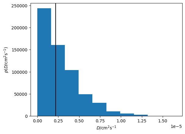
Additionally, we can visualise the distribution of the diffusion coefficient that has been determined.
[16]:
plt.hist(loaded_diff.D_J.samples, density=True)
plt.axvline(loaded_diff.D_J.n, c='k')
plt.xlabel('$D$/cm$^2$s$^{-1}$')
plt.ylabel('$p(D$/cm$^2$s$^{-1})$')
plt.show()
Or the joint probability distribution for the diffusion coefficient and intercept.
[17]:
from corner import corner
[18]:
corner(loaded_diff.flatchain, labels=['$D$/cm$^2$s$^{-1}$', 'intercept/Å$^2$'])
plt.show()
[ ]:
