Comparison with MDAnalysis

MDAnalysis also contains a tool for calculating the mean-squared displacements. So why use kinisi over MDAnalysis?

Well, the approach taken by kinisi, which is outlined in the methodology, uses a high precision approach to estimate the diffusion coefficent and offers an accurate estimate of the variance in the mean-squared displacements and diffusion coefficient from a single simulation.

In this notebook, we will compare the results from MDAnalysis and kinisi. First we will import the kinisi.analyze.DiffusionAnalyzer and MDAnalysis.analysis.msd classes.

import warnings

warnings.filterwarnings('ignore', category=DeprecationWarning)
warnings.filterwarnings('ignore', category=RuntimeWarning)
warnings.filterwarnings('ignore', category=UserWarning)

import numpy as np

import kinisi
from kinisi.analyze import DiffusionAnalyzer
import MDAnalysis.analysis.msd as msd
from MDAnalysis.transformations.nojump import NoJump

Next, we are going to need to do a little ‘magic’ to get MDAnalysis to read an extended xyz file. Luckly ASE can help us out.

from ase.io import read
from MDAnalysis import Universe
import os

Since this trajectory has a triclinic cell; we need to extract the cell dimensions and pass them to MDAnalysis.

# The file we want to load is in the test cases for kinisi, so will need to get the path to it.
path_to_file = os.path.join(os.path.dirname(kinisi.__file__), 'tests/inputs/LiPS.exyz')
atoms = read(path_to_file, format='extxyz', index=':')

cell_dimensions = []
for frame in atoms:
    lengths = frame.cell.lengths()
    angles = frame.cell.angles()
    cell = [*lengths, *angles]
    cell_dimensions.append(cell)

We now have the cell dimensions (\(a, b, c, \alpha, \beta, \gamma\)) in an array. We now need to create an MDAnalysis universe and apply these dimension to it.

u = Universe(path_to_file, path_to_file, format='XYZ', topology_format='XYZ', dt=20.0/1000)
for ts, dims in zip(u.trajectory, cell_dimensions):
    ts.dimensions = dims

Now we add an unwrapping transformation to the universe, create the MSD object, run the analysis, and extract the results as a timeseries.

u.trajectory.add_transformations(NoJump())
MSD = msd.EinsteinMSD(u, select='type LI', msd_type='xyz', fft=True, verbose=False)
MSD.run(verbose=False)
mda_MSD = MSD.results.timeseries

100%|██████████| 896/896 [00:00<00:00, 6652.22it/s]

With the result from MDAnalysis in one hand we can now do the same thing in kinisi with the other. We can also extract the series of \(\Delta t\) from kinisi.

params = {'specie': 'LI',
          'time_step': 0.001,
          'step_skip': 20,
          'n_steps': 250,
          'sampling': 'multi-origin',
          'progress': False}

xyz = {'dimension': 'xyz', 'bootstrap': False,'progress': False}
kinisi_from_universe = DiffusionAnalyzer.from_universe(u, parser_params=params, uncertainty_params=xyz)
kinisi_MSD = kinisi_from_universe.msd
time = kinisi_from_universe.dt

Putting the two analyses’ together, we can plot for comparison.

import matplotlib.pyplot as plt

plt.plot(time[:-1], kinisi_MSD[:-1], label='Kinisi MSD with multi_origin', c='#ff7f0e')
plt.plot(time[:-1], mda_MSD[1:], label='MDanalysis', ls='--')
plt.ylabel('MSD (Å$^2$)')
plt.xlabel('Diffusion time (ps)')
plt.legend()


plt.show()

The results overlap almost entirely.

We can now extract an accurate estimation of the variance in the observed MSD from kinisi. For clarity, we will use array indexing to remove every other data point.

plt.errorbar(kinisi_from_universe.dt[::2],
             kinisi_from_universe.msd[::2],
             kinisi_from_universe.msd_std[::2],
             c='#ff7f0e')
plt.ylabel(r'MSD/Å$^2$')
plt.xlabel(r'$\Delta t$/ps')
plt.show()

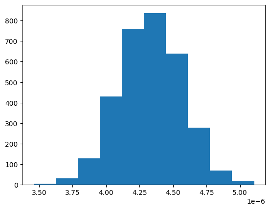
We can also calculate estimated diffusion coefficient, and the associated uncertainty, with kinisi.

from uncertainties import ufloat

kinisi_from_universe.diffusion(kinisi_from_universe.ngp_max)
print('D from kinisi:',
      ufloat(np.mean(kinisi_from_universe.D),
         np.std(kinisi_from_universe.D, ddof=1)))

Likelihood Sampling: 100%|██████████| 1500/1500 [00:01<00:00, 919.22it/s]

D from kinisi: (4.38+/-0.23)e-06