Comparison with pymatgen

The pymatgen project also has tools capable of calculating the mean-squared displacement and diffusion coefficient from a relevant input. So why should you use kinisi over pymatgen?

The simple answer is that the approach taken by kinisi, which is outlined in the methodology, uses a higher precision approach to estimate the diffusion coefficent and offers an accurate estimate in the variance of the mean-squared displacements and diffusion coefficient from a single simulation.

In this notebook, we will compare the results from pymatgen and kinisi. First we will import the kinisi and pymatgen DiffusionAnalyzer classes.

import numpy as np
import matplotlib.pyplot as plt
import scipp as sc
from kinisi.analyze import DiffusionAnalyzer as KinisiDiffusionAnalyzer
from pymatgen.analysis.diffusion.analyzer \
    import DiffusionAnalyzer as PymatgenDiffusionAnalyzer
from pymatgen.io.vasp import Xdatcar
np.random.seed(42)
rng = np.random.RandomState(42)

The kinisi.DiffusionAnalyzer and pymatgen.DiffusionAnalyzer are very similar, but pymatgen does not use scipp to handle dimensions. Pymatgen therefore takes the same imputs, but in in a different format, assuming fs as unit for time. We will define the pymatgen input parameters as p_params.

p_params = {'specie': 'Li',
            'time_step': 2.0,
            'step_skip': 50
            }

xd = Xdatcar('./example_XDATCAR.gz')

We parse Xdatcar.structures to pymatgen to run the analysis. pymatgen also requires an additional temperature keyword.

pymatgen_diff = PymatgenDiffusionAnalyzer.from_structures(
    xd.structures, temperature=300, **p_params)

We can set up the kinisi analysis as in this previous example.

params = {'specie': 'Li',
          'time_step': 2.0 * sc.Unit('fs'),
          'step_skip': 50 * sc.Unit('dimensionless'),
          'progress': False
          }

kinisi_diff = KinisiDiffusionAnalyzer.from_xdatcar(xd, **params)

Now we can plot the mean-squared displacement from each to check agreement.

fig, ax = plt.subplots()

ax.plot(pymatgen_diff.dt, pymatgen_diff.msd, label='pymatgen')
ax.plot(kinisi_diff.dt.values, kinisi_diff.msd.values, label='kinisi')
ax.legend()
ax.set_xlabel(f'Time / {kinisi_diff.dt.unit}')
ax.set_ylabel(f'MSD / {kinisi_diff.msd.unit}')
ax.set_xlim(0, None)
ax.set_ylim(0, None)
plt.show()

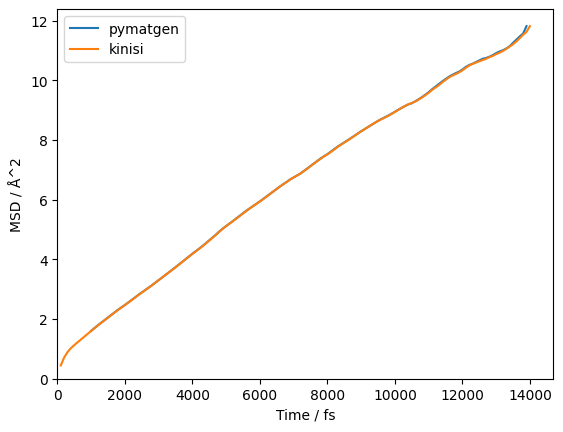
We can see that the results overlap almost entirely.

However, this doesn’t show the benefits for using kinisi over pymatgen. The first benefit is that kinisi will accurately estimate the variance in the observed mean-squared displacements, giving error bars for the above plot.

fig, ax = plt.subplots()

ax.errorbar(kinisi_diff.dt.values,
            kinisi_diff.msd.values,
            np.sqrt(kinisi_diff.msd.variances),
            c='#ff7f0e')
ax.set_xlabel(f'Time / {kinisi_diff.dt.unit}')
ax.set_ylabel(f'MSD / {kinisi_diff.msd.unit}')
ax.set_xlim(0, None)
ax.set_ylim(0, None)
plt.show()

The second benefit is that kinisi will estimate the diffusion coefficient with an accurate uncertainty. pymatgen also estimates this uncertainty, however, pymatgen assumes that the data is independent and applies weighted least squares. However, mean-squared displacement observations are inherently dependent (as discussed in the thought experiment in the methodology), so kinisi accounts for this and applied a generalised least squares style approach. This means that the estimated variance in the diffusion coefficient from kinisi is accurate (while, pymatgen will heavily underestimate the value) and given the BLUE nature of the GLS approach, kinisi has a higher probability of determining a value for the diffusion coefficient closer to the true diffusion coefficient.

start_of_diffusion = 3000 * sc.Unit('fs')
kinisi_diff.diffusion(start_of_diffusion, progress=False, random_state=rng)

from uncertainties import ufloat

print('D from pymatgen:',
      ufloat(pymatgen_diff.diffusivity, pymatgen_diff.diffusivity_std_dev))

D from pymatgen: (1.33307+/-0.00008)e-05

kinisi_diff.D

kinisi.Samples

• • (samples: 3200)
    float64
    cm^2/s
    (1.23+/-0.10)e-05

    Values:
    array([1.25842970e-05, 1.14744119e-05, 1.07672134e-05, ...,
           1.34584966e-05, 1.20766342e-05, 1.31995317e-05], shape=(3200,))

The comparison between weighted and generalised least squared estimators will be discussed in full in a future publication covering the methodology of kinisi.