Investigation of an Arrhenius relationship#
In addition to being able to determine the mean-squared displacement and diffusion coefficient from a given simulation, kinisi also includes tools to investigate Arrhenius relationships. In this tutorial, we will look at how we can take advantage of these tools to study short, approximately 50 ps, simulations of lithium lanthanum zirconium oxide (LLZO).
Warning
The warnings that are being ignored are related to the parsing of the files by MDAnalysis and lead to unnecessary print out to the screen that we want to avoid in the web documentation.
[1]:
import numpy as np
import scipp as sc
import MDAnalysis as mda
import matplotlib.pyplot as plt
from kinisi.analyze import DiffusionAnalyzer
from kinisi.arrhenius import Arrhenius
import warnings
np.random.seed(42)
warnings.filterwarnings("ignore", category=UserWarning)
warnings.filterwarnings("ignore", category=RuntimeWarning)
/home/docs/checkouts/readthedocs.org/user_builds/kinisi/envs/stable/lib/python3.12/site-packages/tqdm/auto.py:21: TqdmWarning: IProgress not found. Please update jupyter and ipywidgets. See https://ipywidgets.readthedocs.io/en/stable/user_install.html
  from .autonotebook import tqdm as notebook_tqdm
To investigate this we will loop through a series of four temperatures and store each mean and variance of the diffusion coefficient in a dictionary.
[2]:
temperatures = np.array([500, 600, 700, 800])
D = {'mean': [], 'var': []}
To read these simulations we will use MDAnalysis (however, it is also possible to use any kinisi.Parser). The parameters are defined for all simulations, here we only consider the diffusive regime to begin after 10 ps.
[3]:
params = {'specie': 'LI',
            'time_step': 5.079648e-4 * sc.Unit('ps'),
            'step_skip': 100 * sc.units.dimensionless,
            'progress': False}
File parsing and diffusion determination is then performed in a loop here.
[4]:
for t in temperatures:
    u = mda.Universe(f'_static/traj_{t}.gro', f'_static/traj_{t}.xtc')
    d = DiffusionAnalyzer.from_universe(u, **params)
    d.diffusion(10 * sc.Unit('ps'), progress=False)
    D['mean'].append(sc.mean(d.D).value)
    D['var'].append(sc.var(d.D, ddof=1).value)
    unit = sc.mean(d.D).unit
We can then use the diffusion coefficients and their variances can be used along with the array of temperatures to create a scipp.DataArray.
[5]:
td = sc.DataArray(
    data=sc.array(dims=['temperature'],
                  values=D['mean'],
                  variances=D['var'],
                  unit=unit,),
    coords={
        'temperature': sc.Variable(dims=['temperature'],
                                   values=temperatures,
                                   unit='K')
    })
td
[5]:
- temperature: 4
- temperature(temperature)int64K500, 600, 700, 800
Values:
array([500, 600, 700, 800])
- (temperature)float64cm^2/s2.163e-06, 2.841e-06, 4.255e-06, 6.515e-06σ = 1.488e-07, 1.964e-07, 2.609e-07, 3.404e-07
Values:
array([2.16277532e-06, 2.84118179e-06, 4.25458330e-06, 6.51504324e-06])

Variances (σ²):
array([2.21312627e-14, 3.85875677e-14, 6.80722775e-14, 1.15896219e-13])
With the DataArray created, we can now create the Arrhenius object.
[6]:
s = Arrhenius(td, bounds=[[0.1 * sc.Unit('eV'), 0.2 * sc.Unit('eV')],
                          [1e-5 * td.data.unit, 1e-4 * td.data.unit]])
When you create a TemperatureDependent object, of which Arrhenius is a subclass, you can optionally provide bounds as a list of lists. For example, if we wanted the activation energy to be restricted between 0.1 and 0.2 eV and the preexponential factor between 10-5 and 10-4 cm2/s, then we would use the following:
Arrhenius(td, bounds=[[0.1 * sc.Unit('eV'), 0.2 * sc.Unit('eV')],
                      [1e-5 * td.data.unit, 1e-4 * td.data.unit]])
If you do not set bounds, they are automatically set to 0.5 and 1.5 of the best fit values.
The Arrhenius object automatically estimates the maximum likelihood values for the activation energy and preexponential factor and stores them is an appropriate sc.DataGroup.
[7]:
s
[7]:
- datascippDataArray(temperature: 4)float64cm^2/s2.163e-06, 2.841e-06, 4.255e-06, 6.515e-06
- activation_energyscippVariable()float64eV0.1297575166747647
- preexponential_factorscippVariable()float64cm^2/s3.916136406276413e-05
However, kinisi also allows us to estimate the full distribution of these parameters with Markov chain Monte Carlo (MCMC) sampling.
[8]:
s.mcmc()
MCMC Sampling: 100%|██████████| 1500/1500 [00:19<00:00, 78.93it/s]
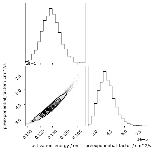
We can then visualise the probability distributions for the parameters as histograms.
[9]:
from corner import corner
[10]:
corner(np.array([i.values for i in s.flatchain.values()]).T,
       labels=[' / '.join([k, str(v.unit)]) for k, v in s.flatchain.items()])
plt.show()
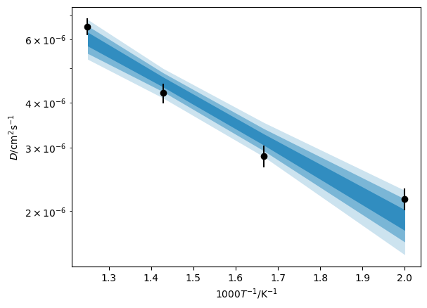
It is also possible to plot these probability distributions as Arrhenius relations on the data measured values.
[11]:
credible_intervals = [[16, 84], [2.5, 97.5], [0.15, 99.85]]
alpha = [0.6, 0.4, 0.2]

plt.errorbar(1000/td.coords['temperature'].values,
             td.data.values,
             np.sqrt(td.data.variances),
             marker='o',
             ls='',
             color='k',
             zorder=10)

for i, ci in enumerate(credible_intervals):
    plt.fill_between(1000/td.coords['temperature'].values,
                     *np.percentile(s.distribution, ci, axis=1),
                     alpha=alpha[i],
                     color='#0173B2',
                     lw=0)
plt.yscale('log')
plt.xlabel('$1000T^{-1}$/K$^{-1}$')
plt.ylabel('$D$/cm$^2$s$^{-1}$')
plt.show()
Finally, the activation energy and preexponential factor are kinisi.samples.Samples objects and are stored in the Arrhenius object.
[12]:
s.activation_energy
[12]:
- (samples: 3200)float64eV0.133+/-0.011
Values:
array([0.1359232 , 0.11996698, 0.12375936, ..., 0.12492265, 0.12010634,
       0.13609629], shape=(3200,))
[13]:
s.preexponential_factor
[13]:
- (samples: 3200)float64cm^2/s(4.2+/-0.8)e-05
Values:
array([4.40815129e-05, 3.24628711e-05, 3.41540489e-05, ...,
       3.51212315e-05, 3.25081681e-05, 4.40273586e-05], shape=(3200,))