Diffusion coefficient of molecules using center of mass#
Kinisi includes the ability to calculate the mean-squared displacement and diffusion coefficient of the center of mass (or geometry) of molecules. This can be done for a single molecule or a collection of molecules. It is important to note that inclusion of rotational motion in the calcuation of diffusion coeffiencents can lead to erronious results. This rotation can be elminated from the calculation by taking the center of mass for each molecule.
[1]:
import numpy as np
from ase.io import read
import matplotlib.pyplot as plt
from kinisi.analyze import DiffusionAnalyzer
import scipp as sc
We will use a simulation of ethene in ZSM-5 zeolite. This was run in DL_POLY, so we will use ASE to load in the trajectory (HISTORY) file.
[2]:
traj = read('ethene_zeo_HISTORY.gz', format='dlp-history', index=':')
We want to calculate the diffusion of the center of mass of the ethene molecule. This can be done by setting specie to None and specifying the indices of the molecules of interest in specie_indices as a scipp array. To define molecules, a scipp array should be passed under the specie_indices keyword with two dimensions atom and group_of_atoms.
The particle dimension should be the same size as the number of molecules, particle is the generic term in kinisi for a particle or group of particles.
The atoms in particle dimension should be the same size as the number of atoms in each each molecule.
In the example below we are calculating the msd and diffusion for 2 ethene molecules.
Only identical molecules are supported. The masses of the atoms in the molecules can be specified with masses. This must be a scipp array with the same length and dimension atoms in particle as a molecule.
[3]:
molecules = [[288, 289, 290, 291, 292, 293],
             [284, 295, 296, 297, 298, 299]]
mass    =  [12, 12, 1.008, 1.008, 1.008, 1.008]

params = {'specie': None,
           'time_step': 1.2e-03 * sc.Unit('ps'),
           'step_skip': 100 * sc.Unit('dimensionless'),
           'specie_indices': sc.array(dims=['particle', 'atoms in particle'],
                                      values=molecules,
                                      unit=sc.Unit('dimensionless')),
           'masses': sc.array(dims = ['atoms in particle'],
                              values = mass),
           'progress': False
           }
With the parameters set, we now calcuate the mean squared-displacement.
[4]:
diff = DiffusionAnalyzer.from_ase(traj, **params)
[5]:
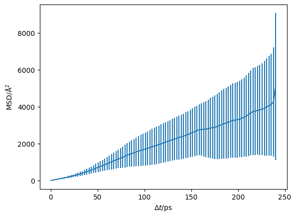
plt.errorbar(diff.dt.values[::20],
             diff.msd.values[::20],
             diff.msd.variances[::20]**0.5)
plt.ylabel('MSD/Å$^2$')
plt.xlabel(r'$\Delta t$/ps')
plt.show()
[6]:
start_of_diffusion = 60 * sc.Unit('ps')
diff.diffusion(start_of_diffusion, progress = False)
[7]:
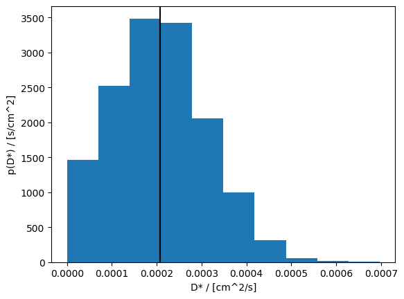
diff.D
[7]:
- (samples: 3200)float64cm^2/s0.00021+/-0.00011
Values:
array([9.50661138e-05, 1.95346964e-04, 3.52187252e-04, ...,
       1.17227790e-04, 1.19361809e-04, 1.67313515e-04], shape=(3200,))
[8]:
fig, ax = plt.subplots()

ax.hist(diff.D.values, density=True)
ax.axvline(sc.mean(diff.D).value, c='k')
ax.set_xlabel(f'D* / [{diff.D.unit}]')
ax.set_ylabel(f'p(D*) / [{(1 / diff.D.unit).unit}]')
plt.show()
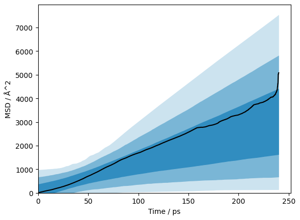
[9]:
credible_intervals = [[16, 84], [2.5, 97.5], [0.15, 99.85]]
alpha = [0.6, 0.4, 0.2]

fig, ax = plt.subplots()
ax.plot(diff.dt.values, diff.msd.values, 'k-')
for i, ci in enumerate(credible_intervals):
    ax.fill_between(diff.dt.values,
                      *np.percentile(diff.distributions, ci, axis=1),
                      alpha=alpha[i],
                      color='#0173B2',
                      lw=0)
ax.set_xlabel(f'Time / {diff.dt.unit}')
ax.set_ylabel(f'MSD / {diff.msd.unit}')
ax.set_xlim(0, None)
ax.set_ylim(0, None)
plt.show()