Handling a poorly conditioned covariance matrix#
Sometimes, you may end up with a very clearly incorrect result from kinisi. For example, consider the MSD plot below.
[1]:
import os
import numpy as np
import scipp as sc
import kinisi
from kinisi.analyze import DiffusionAnalyzer
from ase.io import read
from MDAnalysis import Universe
import matplotlib.pyplot as plt

credible_intervals = [[16, 84], [2.5, 97.5], [0.15, 99.85]]
alpha = [0.6, 0.4, 0.2]

path_to_file = os.path.join(os.path.dirname(kinisi.__file__),
                            'tests/inputs/LiPS.exyz')
atoms = read(path_to_file, format='extxyz', index=':')

cell_dimensions = []
for frame in atoms:
    lengths = frame.cell.lengths()
    angles = frame.cell.angles()
    cell = [*lengths, *angles]
    cell_dimensions.append(cell)

u = Universe(path_to_file,
             path_to_file,
             format='XYZ',
             topology_format='XYZ',
             dt=20.0/1000)
for ts, dims in zip(u.trajectory, cell_dimensions):
    ts.dimensions = dims

params = {'specie': 'LI',
          'time_step': 0.001 * sc.Unit('ps'),
          'step_skip': 20 * sc.units.dimensionless,
          'progress': False
          }

diff = DiffusionAnalyzer.from_universe(u, **params)
diff.diffusion(1.5 * sc.Unit('ps'))

fig, ax = plt.subplots()
ax.plot(diff.dt.values, diff.msd.values, 'k-')
for i, ci in enumerate(credible_intervals):
    ax.fill_between(diff.dt.values,
                      *np.percentile(diff.distributions, ci, axis=1),
                      alpha=alpha[i],
                      color='#0173B2',
                      lw=0)
ax.set_xlabel(f'Time / {diff.dt.unit}')
ax.set_ylabel(f'MSD / {diff.msd.unit}')
ax.set_xlim(0, None)
ax.set_ylim(0, None)
plt.show()
/home/docs/checkouts/readthedocs.org/user_builds/kinisi/envs/stable/lib/python3.12/site-packages/tqdm/auto.py:21: TqdmWarning: IProgress not found. Please update jupyter and ipywidgets. See https://ipywidgets.readthedocs.io/en/stable/user_install.html
  from .autonotebook import tqdm as notebook_tqdm
Likelihood Sampling: 100%|██████████| 1500/1500 [00:01<00:00, 1279.96it/s]
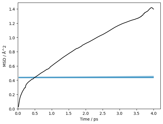
Obviously something has gone wrong in this analysis. Unfortunately, this issue arises due to the numerical precision of computers, and there really isn’t much that can be done to stop it. However, we can work around this issue.
This problem arises due to the condition number of the covariance matrix being very high.
[2]:
np.linalg.cond(diff.diff.covariance_matrix.values)
[2]:
np.float64(2.392934289306048e+16)
This means that when the matrix is inverted, the result is very sensitive to small changes, on the scale of machine precision.
kinisi tries its best to make sure that the matrix has a low enough condition number that this doesn’t happen. But unfortunately, it is not always possible to achieve a low enough condition number. Therefore, we need to find a different solution.
So far, the best solution that we have found has been to recondition the matrix in an effort to reduce the noise. We are working on a full assessment of the effectiveness of this approach and hope to have a preprint on the subject soon. To use the reconditioning, run.
[3]:
diff.diffusion(1.5 * sc.Unit('ps'), recondition=True)

fig, ax = plt.subplots()
ax.plot(diff.dt.values, diff.msd.values, 'k-')
for i, ci in enumerate(credible_intervals):
    ax.fill_between(diff.dt.values,
                      *np.percentile(diff.distributions, ci, axis=1),
                      alpha=alpha[i],
                      color='#0173B2',
                      lw=0)
ax.set_xlabel(f'Time / {diff.dt.unit}')
ax.set_ylabel(f'MSD / {diff.msd.unit}')
ax.set_xlim(0, None)
ax.set_ylim(0, None)
plt.show()
Likelihood Sampling: 100%|██████████| 1500/1500 [00:01<00:00, 1213.56it/s]
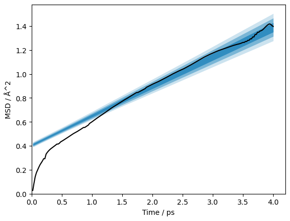
You will notice that this can significantly reduce the condition number.
[4]:
np.linalg.cond(diff.diff.covariance_matrix.values)
[4]:
np.float64(518.2354688998988)
However, this is not always successful. The next approach to resolve this issue is to change the time intervals, dt, that is used. Because we estimate the full covariance matrix, within reason, computing the MSD at every possible time interval is usually overkill. Instead, we can use a longer time interval sets, currently the time intervals are 0.02 ps apart.
[5]:
diff.dt
[5]:
- (time interval: 200)float64ps0.02, 0.04, ..., 3.980, 4.0
Values:
array([0.02, 0.04, 0.06, 0.08, 0.1 , 0.12, 0.14, 0.16, 0.18, 0.2 , 0.22,
       0.24, 0.26, 0.28, 0.3 , 0.32, 0.34, 0.36, 0.38, 0.4 , 0.42, 0.44,
       0.46, 0.48, 0.5 , 0.52, 0.54, 0.56, 0.58, 0.6 , 0.62, 0.64, 0.66,
       0.68, 0.7 , 0.72, 0.74, 0.76, 0.78, 0.8 , 0.82, 0.84, 0.86, 0.88,
       0.9 , 0.92, 0.94, 0.96, 0.98, 1.  , 1.02, 1.04, 1.06, 1.08, 1.1 ,
       1.12, 1.14, 1.16, 1.18, 1.2 , 1.22, 1.24, 1.26, 1.28, 1.3 , 1.32,
       1.34, 1.36, 1.38, 1.4 , 1.42, 1.44, 1.46, 1.48, 1.5 , 1.52, 1.54,
       1.56, 1.58, 1.6 , 1.62, 1.64, 1.66, 1.68, 1.7 , 1.72, 1.74, 1.76,
       1.78, 1.8 , 1.82, 1.84, 1.86, 1.88, 1.9 , 1.92, 1.94, 1.96, 1.98,
       2.  , 2.02, 2.04, 2.06, 2.08, 2.1 , 2.12, 2.14, 2.16, 2.18, 2.2 ,
       2.22, 2.24, 2.26, 2.28, 2.3 , 2.32, 2.34, 2.36, 2.38, 2.4 , 2.42,
       2.44, 2.46, 2.48, 2.5 , 2.52, 2.54, 2.56, 2.58, 2.6 , 2.62, 2.64,
       2.66, 2.68, 2.7 , 2.72, 2.74, 2.76, 2.78, 2.8 , 2.82, 2.84, 2.86,
       2.88, 2.9 , 2.92, 2.94, 2.96, 2.98, 3.  , 3.02, 3.04, 3.06, 3.08,
       3.1 , 3.12, 3.14, 3.16, 3.18, 3.2 , 3.22, 3.24, 3.26, 3.28, 3.3 ,
       3.32, 3.34, 3.36, 3.38, 3.4 , 3.42, 3.44, 3.46, 3.48, 3.5 , 3.52,
       3.54, 3.56, 3.58, 3.6 , 3.62, 3.64, 3.66, 3.68, 3.7 , 3.72, 3.74,
       3.76, 3.78, 3.8 , 3.82, 3.84, 3.86, 3.88, 3.9 , 3.92, 3.94, 3.96,
       3.98, 4.  ])
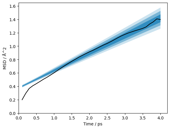
We will reduce that so there is 0.1 ps between the time intervals, which we can do by setting a custom set of time intervals.
[6]:
new_dt = sc.arange(dim='time interval', start=0.1 * sc.Unit('ps'),
                   stop=4.1 * sc.Unit('ps'),
                   step=0.1 * sc.Unit('ps'))
The new dt must be a subset of the old dt values, the cell below checks this.
[7]:
print(np.all(np.any(np.isclose(new_dt.values[:, None],
                               diff.dt.values[None, :]),
                    axis=1)))

params['dt'] = new_dt
True
Running this through again, we can see that we get a much more reasonable value.
[8]:
diff = DiffusionAnalyzer.from_universe(u, **params)
diff.diffusion(1.5 * sc.Unit('ps'))

fig, ax = plt.subplots()
ax.plot(diff.dt.values, diff.msd.values, 'k-')
for i, ci in enumerate(credible_intervals):
    ax.fill_between(diff.dt.values,
                      *np.percentile(diff.distributions, ci, axis=1),
                      alpha=alpha[i],
                      color='#0173B2',
                      lw=0)
ax.set_xlabel(f'Time / {diff.dt.unit}')
ax.set_ylabel(f'MSD / {diff.msd.unit}')
ax.set_xlim(0, None)
ax.set_ylim(0, None)
plt.show()
Likelihood Sampling: 100%|██████████| 1500/1500 [00:01<00:00, 1359.42it/s]
We welcome any user feedback on this problem, i.e., if you have a better way to mitigate it or remove it completely.